Miniproject 2: Beach Muscles

Introduction

Our musculoskeletal system is pretty handy in permitting us to move, hold, or manipulate objects, including our own bodies. Many vertebrate biomechanical systems make use of muscular force applied to levers in order to resists or overcome these loads. In this MP, we’ll explore a classic lever system in the tetrapod body—the forelimb—one of the 3rd-order type. Specifically, we’ll consider how skeletal geometry and important physiological parameters, like muscle length and mass, affect the force output in this system and maximum load it can support.

To begin, let’s assume the following.

All the force to do the lift is exerted by your biceps femoralis
The weight in the palm of your hand
Your humerus is stationary
The elbow joint is a simple hinge linkage with one DOF
The flexion of the arm (i.e., curl motion) begins when your arm angle is 150$^\circ$ and is finished at 50$^\circ$.

What we have here, according to a classic concept in physics, is a dynamic equilibrium problem. That is, if the sum of torques is not zero, the mass of the dumbbell will be accelerated, a situation described by:

\[ \alpha=\frac{\Sigma\tau}{I}, \]

where $\alpha$ is angular acceleration (in rad$\cdot$s$^{-2}$), $\Sigma\tau$ is sum of torques (N$\cdot$m), and $I$ is the mass moment of inertia (in kg$\cdot$m$^2$). Or, if $\tau_{muscle}$ represents muscle torque and $\tau_{load}$ the load tourque, we have

\[ \alpha=\frac{\tau_{muscle}-\tau_{load}}{I}. \]

This is the rotational application of Newton’s Second Law. We can simplify our problem it we consider that, under equilibrium, $\alpha=0$. Therefore, under equilibirium, $\tau_{muscle}=\tau_{load}$

Based on these concepts, our task in this MP is to calculate how much torque ($\tau$) is generated at the outlever position of the arm system.

The specific goals are to:

Predict how much force and torque is produced by the biceps system over a range of extension/flexion angels.
Assess how force and torque vary according to extension/flexion angle.
Test these predictions in the gym.

Methods

We’ll approach this problem by constructing a computational model based on dynamic equilibrium, one that includes some very important muscle and geometric parameters. We’ll model arm torque output over a range of arm extension/flexion angles, from nearly fully extended (extension angle of 150$^\circ$) to fully flexed arm (extension angle of 50$^\circ$). This will include extension angles of 50, 75, 100, 125, and 150$^\circ$).

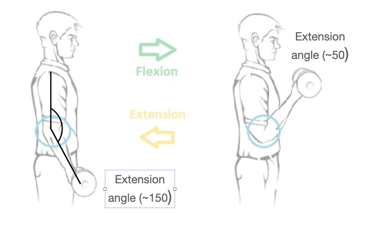
Fig. 1: The human elbow lever at full extension and flexion.

## ── Attaching core tidyverse packages ──────────────────────── tidyverse 2.0.0 ──
## ✔ dplyr     1.1.4     ✔ readr     2.1.4
## ✔ forcats   1.0.0     ✔ stringr   1.5.1
## ✔ ggplot2   3.4.4     ✔ tibble    3.2.1
## ✔ lubridate 1.9.2     ✔ tidyr     1.3.0
## ✔ purrr     1.0.2     
## ── Conflicts ────────────────────────────────────────── tidyverse_conflicts() ──
## ✖ dplyr::filter() masks stats::filter()
## ✖ dplyr::lag()    masks stats::lag()
## ℹ Use the conflicted package (<http://conflicted.r-lib.org/>) to force all conflicts to become errors

The lever model

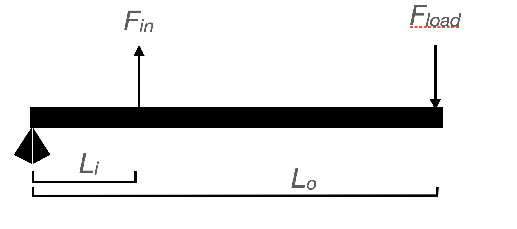
Fig. 2: The moments applied to a 3d order lever

When in equilibrium (i.e., no rotational motion, Figure 2), the sum of torques applied to a lever system like one of the 3rd order variety shown above are equal. That is, $F_i \cdot L_i = F_{load} \cdot L_o$. Or, in terms of our 3rd order arm system, $F_{muscle} \cdot L_i = F_{load} \cdot L_o$.

This assumes that both forces, $F_{muscle}$ and $F_{Load}$ are applied normal to the lever system, that is at a perfect 90$^\circ$ angle. For our system, the geometry of which is presented below in Figure 3, let’s assume the load is in the palm, resting directly on the outlever and thus the angle of the load $F_{load}$ is normal. The insertion angle of the muscle relative to the inlever of the formarm $\theta$ is not normal and, in fact, changes with extension/flexion angle as seen in Figure 4.

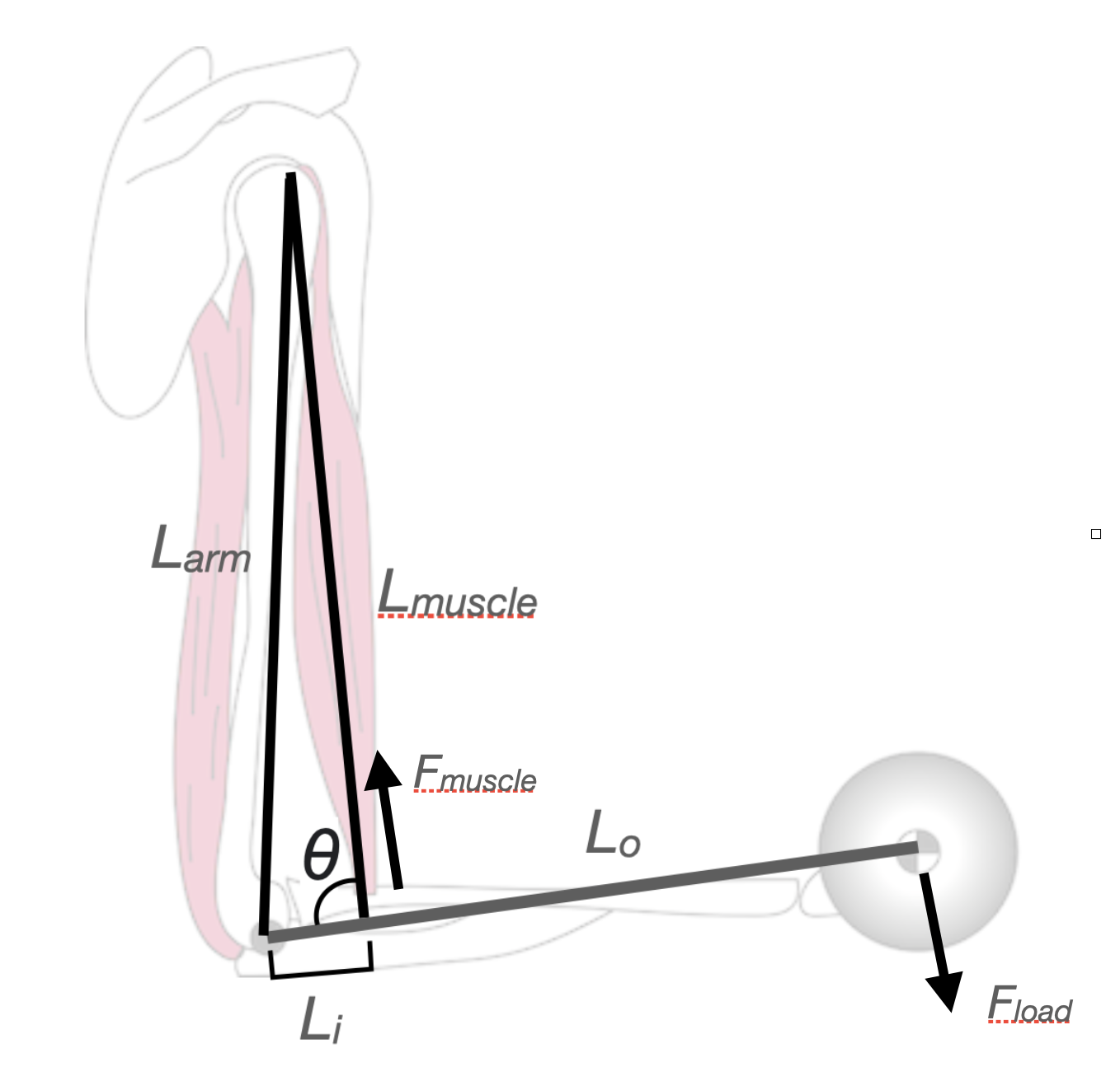
Fig. 3: The human elbow lever.

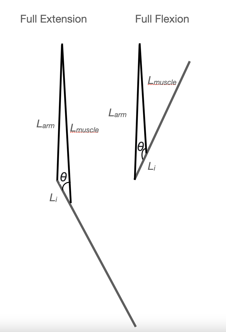
$Fig. 4: The human elbow lever at full extension and flexion. Notice how the insertion angle and $L_{muscle}$ change$

Fig. 4: The human elbow lever at full extension and flexion. Notice how the insertion angle and $L_{muscle}$ change

Therefore, the torque applied my a muscle to the lever ($\tau_{muscle}$) is also function of the insertion angle, in addition to $F_{muscle}$ and $L_i$, or

\[ \tau_{muscle}=F_{muscle} \cdot sin\theta \cdot L_i. \]

Determining $F_{muscle}$

From this or previous explorations of muscle physiology, we now know that the amount of force produced by a muscle is a function of time (i.e., latency), shortening velocity, and muscle length. Because we’re applying an equilibrium model to our lever system, there will be no rotation and therefore no changes in muscle length at each arm postion. This means an isometric contraction and a muscle with no velocity. So, we don’t have to consider the force-velocity relationship. We can ignore latency in our model, logically assuming our contractions will last longer thant the 20–50 ms before peak muscle force.

However, one of these factors, muscle length, is a factor and an extremely important part of Hill-type muscle models (Hill 1938) like the one we’re constructing

To do this we must establish the relationship between the muscle length and the maximum amount of force a muscle can produce ($F_{max}$), also called the force-length factor or $f_{fl}$. Fortunately, the relationship between force and muscle length has been approximated for mammalian skeletal muscle by several researchers, including (Whiting and Herzog 1999), from whence the following comes. It looks a bloody mess, but here it is:

\[f_{fl}=-6.25\Bigg(\cfrac{L_{muscle}}{L_{opt}}\Bigg)^2+12.5\Bigg(\cfrac{L_{muscle}}{L_{opt}}\Bigg)-5.25,\]

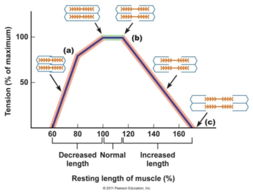
Fig. 5: The force-length relationship of vertebrate muscle

where $L_{opt}$ is the optimal muscle length. So, ``What is the optimal muscle length?” you ask. Well, we don’t know, not exactly. But, a lot of good experimental work suggests that, for many muscles in many species, it’s an $L_{muscle}$ that is close to 80% the maximum length. So let’s use that and assume the maximum length of the muscle is reached at rest (i.e., extension angle of 150$^\circ$, $L_{muscle_r}$). Therefore, $L_{opt}= L_{muscle_r} \cdot 0.8$.

As you can see from Figure 5, such a value assumes that the muscle is adapted to work over a range of lengths that results in favorable sarcomere overlap. Once we know the we can multiple $F_{max}$ by the factor $f_{fl}$ to estimate how much force is being produced given the muscle’s position of the force-length curve ($F_{muscle}$).

Determining $\theta$

Have a look at the figure of the arm system in Figure 4. For any flexion/extension angle, insertion angle can be computed using the law of cosines. This law states that, for a triangle with length l, r, and o (left, right, and opposite) the angle $\theta$ is:

\[ \theta=acos\Bigg(\cfrac{-o^2+l^2+r^2}{2lr}\Bigg) \]

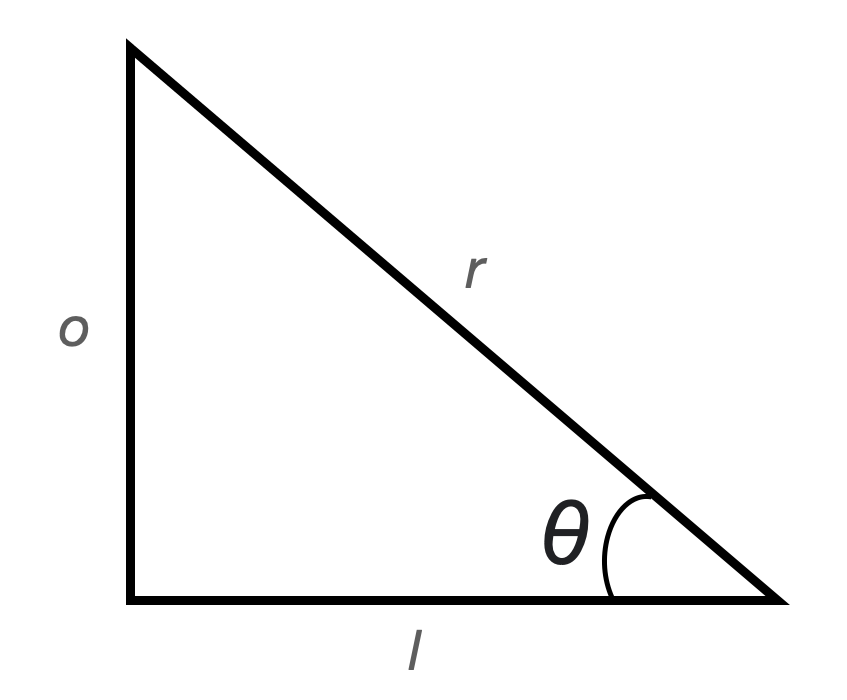
Fig. 6: A triangle

Here, it’s easy to see that $o$ would represent $L_{arm}$, segment $l$ inlever length ($L_{i}$), and segment $r$ the muscle length ($L_{muscle}$).

Please write a function named law_cos that will help you compute $\theta$, the insertion angle. Make sure that the function takes the argumes o,r``, andl`.

Determining $L_{muscle}$

Similarly, muscle length will change with flexion angle and we can use the law of cosines to compute muscle length. Here we just solve for $o$ if we consider a triangle like that in Figure 7. Hoefully you can see that segment $o$ would represent $L_{muscle}$, segment $l$ the arm length ($L_{arm}$), segment $r$ the inlever length ($L_i$), and $theta$ the flexion angle. Doing the algebra, we get:

\[o=\sqrt{-1\cdot(cos(\theta)\cdot 2 \cdot l\cdot r-l^2-r^2)}.\]

Please write a function named law_cos2 that will help you compute $L_{muscle}$ at each flexion angle. Make sure that it includes the arguments l, r, and theta.

Note: You’ll have to do this first, before computing insertion angle. That is, you need $L_{muscle}$ to compute $\theta$.

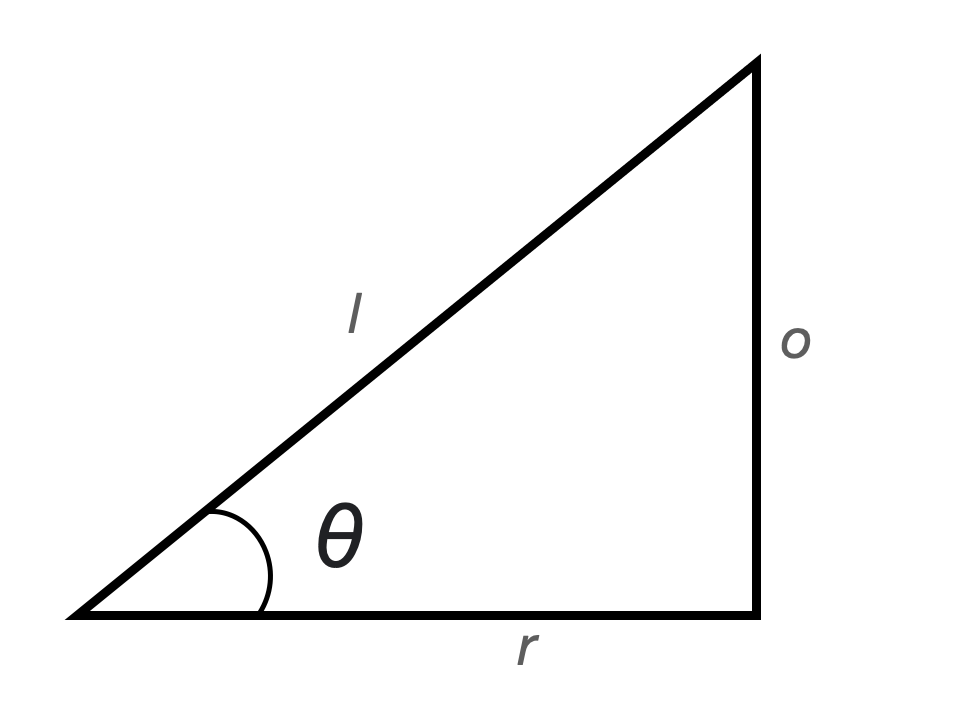
Fig. 7: Another triangle

Determining $F_{max}$

To compute $F_{muscle}$, we must therefore know the $F_{max}$. As we have discussed or will, the amount of force produced by a muscle is is determined by how many crossbridges it can form. This number can be roughly estimated by a muscle’s physiological cross-sectional area (PCSA), a value computed in this way:

\[ PCSA=\cfrac{M_{muscle} \cdot cos(\phi)}{\rho \cdot L_{muscle_r}} \]

where $M_{muscle}$ is the mass of the muscle (in kg), $\phi$ is the pennation angle, $L_{muscle_r}$ the length of the muscle at rest (in cm), and $\rho$ the density of muscle.

When computing the PCSA of your biceps, make following assumptions:

the length of your biceps containing all the fibers is the resting the origin-insertion length, $L_{muscle_r}$, the length at full extension (150$^\circ$);
the density of muscle is 0.00105 kg cm$^{-3}$;
the muscle is nonpennate ($\phi$=0); and lastly
the mass of your muscle is approximated by a volume of playdough.

To estimate the mass of your right biceps with playdough, sculpt the clay to a spheroid that matches the volume of your fully shortened biceps. Flexing and cupping the muscle with your left hand helps with estimating the muscle volume. Next, weigh the playdough (if your muscle mass is large enough, you may have to break the playdough into pieces and way them separately). Vertebrate muscle is about as dense as playdough.

If the maximal force output of human white muscle (the constant $k$) is 80 N cm$^{-2}$ during an isometric contraction (our scenario), you can now compute $F_{max}$

Putting it all together

Let’s assemble all this together. The ammount of tourque the biceps lever system can produce is therefore

\[\tau_{muscle}=\cfrac{M_{muscle} \cdot cos(\phi)}{\rho \cdot L_{muscle_r}}\cdot k \cdot -6.25\Bigg(\cfrac{L_{muscle}}{L_{muscle_r}\cdot 0.8}\Bigg)^2+12.5\Bigg(\cfrac{L_{muscle}}{L_{muscle_r} \cdot 0.8}\Bigg)-5.25\cdot sin(\theta)\cdot L_i \]

Perhaps your head is spinning and you’re not sure where all this comes from. These are just the the components discussed above in long form:

$F_{max}$, the maximum amount of force a muscle can produce determine by PCSA:

\[\cfrac{M_{muscle} \cdot cos(\phi)}{\rho \cdot L_{muscle_r}}\cdot k\]

$f_{fl}$, the force-length factor:

\[-6.25\Bigg(\cfrac{L_{muscle}}{L_{muscle_r} \cdot 0.8}\Bigg)^2+12.5\Bigg(\cfrac{L_{muscle}}{L_{muscle_r} \cdot 0.8}\Bigg)-5.25\]

$sin(\theta)$, the muscle insertion angle.
and $L_i$, the inlever length.

Together, items 1 and 2 make up $F_{muscle$}.

You task is to render all this in repeatable and adjustable computational model as an R function. According to the model, this function should be named model and take as arguments the following:

mass: Muscle mass, $M_{muscle}$, in kg.
Lmuscler: Length of the muscle at rest (150$^\circ$ extension), $L_{muscle_r}$ in m.
Lmuscle: Length of the muscle at any flexion/extension angle, $L_{muscle}$ in m.
theta: Insertion angle of the muscle any flexion/extension angle, $\theta$.
Li: Length of the inlever, $L_i$ in m.
rho: A value for muscle density $\rho$ with a default of 0.00105 kg cm$^{-1}$.
k: A value for $k$, the maximal force output of human white muscle with a default of 80 N cm$^{-2}$.

Note: The PCSA model above depends on lengths in cm. Your computational model must account for this, especially given that our lengths are in m.

The function should also return the predicted torque based on these inputs.

Please apply this model function to the six extension angles: 50, 75, 100, 125, and 150$^\circ$). To begin your calculations, create a tibble that includes the following columns:

flexion: the flexion angles, 50, 75, 100, 125, and 150$^\circ$, but in radians
Lmuscle: the $L_{muscle}$ values at each flexion angle
theta: the insertion angle values ($\theta$) at each flexion angle.

Then, apply the model() function using mutate() and your measured biometric data to add a new column muscle_torque. Call this tibble object dat.

Please also add the predicted load mass your arm system could support. Remember that equilibrium assumes the muscle and load torques are equal. Therefor, you’ll have to find what mass results in a load torque that would equal the muscle torque. For that, $\tau_{load}=\tau_{muscle}$. If

\[\tau_{load}=F_{load} \cdot L_o,\] where $F_{load}$ is the static force of the load and $L_o$ is the outlever length, and

\[F_{load}=M_{load} \cdot g,\] where $M_{load}$ is the mass of the load and $g$ the acceleration due to gravity, we then come to:

\[ M_{load}=\frac{\tau_{muscle}}{L_o \cdot g}.\] Please add $M_{load}$ to your dat table in the column max_mass.

You should wind up with something like this (Prof. K’s data*):

## # A tibble: 6 × 5
##   flexion Lmuscle theta muscle_torque max_mass
##     <dbl>   <dbl> <dbl>         <dbl>    <dbl>
## 1   2.62    0.313 0.428          7.63     4.90
## 2   2.18    0.298 0.795         16.7     10.7 
## 3   1.75    0.277 1.18          26.0     16.7 
## 4   1.31    0.251 1.60          30.2     19.4 
## 5   0.873   0.226 2.06          25.0     16.0 
## 6   0.436   0.207 2.58          13.0      8.34

*His biometric data were:

Variable	Value
$M_{muscle}$	0.207 kg
$L_o$	0.35 m
$L_i$	0.06 m
$L_{arm}$	0.26 m

Model assessment

Now that you know how much torque your biceps can produce based on your arm’s geometry, biceps mass and length, what is the maximum mass (i.e. heaviest weight) you could lift at each position?

The next and last part of this experiment is to test your model. So, skip on over to the largest building on campus and test these theoretical calculations. Find a weight of the closest mass for your calculation for an arm angle that produced large $M_{load}$ value. Go lighter or heavier until you can or can’t accelerate the dumbbell.

Please capture a video showing your attempt at proofing your model Be sure to give it the filename “first_last_plex” Make sure the mass is identified in the video and you isolate the biceps, i.e., no swinging.

Biometric data

To recap, you’ll have to measure several dimension of your arm lever system to feed the model and asses its accuracy. Other values will have to be calculated.

Those to be measured:

Muscle mass ($M_{muscle}$): Do so with the playdough method in the lab.
Arm length ($L_{arm}$): Do so with a meter stick in the lab.
Inlever length ($Li$): Do so with a meter stick in the lab.
Outlever length ($Li$): Do so with a meter stick in the lab.

Those to be calculated:

Muscle lengths at each flexion angle ($L_{muscle}$)
Muscle insertion angle at each flexion angle($\theta$)

What to address in the report

After you recover, please synthesize your results and findings according to the suggested organization for an MP report. Remember, you must cite two relevant primary sources. You can find explicit details concerning the organization of an MP report here.

With this in mind, please address the following:

What were your predicted $\tau_{muscle}$ and $M_{load}$ values at each flexion angle?
Is there any pattern to these values? What explains these patterns?
How did your gym testing compare to your model estimations? That is, was it more or less than predicted?
If the model was produced poor predictions, why?

Be sure to include at least one visualization of your predictions.

Due Date and Submission

Reports are due by Wednesday, February 14st at 11:59 pm. You should compress your directory containing the .Rmd, all class data, and videos of each member assessing the model. This .zip file should be uploaded here.

What to pay attention to in writing the report:

Data are plural
Don’t use print(), head(), etc. commands needlessly
Figure axes should be labelled appropriately.

References

Hill, Archibald Vivian. 1938. “The Heat of Shortening and the Dynamic Constants of Muscle.” Proceedings of the Royal Society of London. Series B-Biological Sciences 126 (843): 136–95.

Whiting, B, and W Herzog. 1999. Theoretical Models of Skeletal Muscle: Biological and Mathematical Considerations. Chichester: Wiley.