AME Example Solution
Prof. K.
2025-02-04
Analysis
Open, save, and establish an R markdown document that includes a YAML header with your name, title, date and output as an html [1].
Include an R chunk that loads
tidyverse[1].
## Warning: package 'ggplot2' was built under R version 4.2.3## ── Attaching core tidyverse packages ── tidyverse 2.0.0 ──
## ✔ dplyr 1.1.1 ✔ readr 2.1.4
## ✔ forcats 1.0.0 ✔ stringr 1.5.0
## ✔ ggplot2 3.5.1 ✔ tibble 3.2.1
## ✔ lubridate 1.9.2 ✔ tidyr 1.3.0
## ✔ purrr 1.0.1
## ── Conflicts ──────────────────── tidyverse_conflicts() ──
## ✖ dplyr::filter() masks stats::filter()
## ✖ dplyr::lag() masks stats::lag()
## ℹ Use the conflicted package (<http://conflicted.r-lib.org/>) to force all conflicts to become errors- Please download the data you see above by accessing this link. Read it in as CSV data and
save it to an object named
dat. [3]
## Rows: 20 Columns: 3
## ── Column specification ──────────────────────────────────
## Delimiter: ","
## chr (1): sex
## dbl (2): mass, Fmax
##
## ℹ Use `spec()` to retrieve the full column specification for this data.
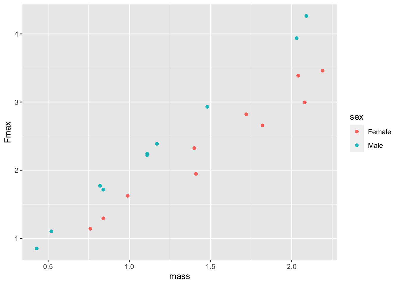
## ℹ Specify the column types or set `show_col_types = FALSE` to quiet this message.- Produce an illustrative visualization of the relationship between squirrel maximum bite force and mass and how this relationship may vary by sex. [3]

Interpretation
Overall, bite force increases with mass while males, on average have higher bite force than females. Perhaps the sexual differences arise due to sexual selection, i.e., males spar with one another in competition for females and over territory.